Parametric drawings with Calcpad

Besides text and formulas, Calcpad allows you to add scaled parametric vector images to your reports. Their dimensions can depend on your input data and the results from the calculations. It means that if you change some values, the drawings will resize accordingly. An example drawing of a prestressed TT panel section, created with Calcpad is given below:

This is obtained by inserting an SVG image in Calcpad and assigning expressions/variables to coordinates instead of fixed values. SVG (Scalable Vector Graphics) is a markup language, based on XML, for defining vector graphics for the web. You can learn more for SVG from this tutorial in W3Schools:

https://www.w3schools.com/graphics/svg_intro.asp

You can keep your SVG image in a separate file or embed it into an Html document. Since Calcpad supports Html inside comments, it automatically supports SVG as well. For convenience, some of the most common SVG elements are included into the “Insert” menu:

You must start with inserting a drawing. When you click the menu, Calcpad will add the following code snippet inside your worksheet:

#val
#hide
w = 400
h = 400
#show
'<svg viewbox="'0' '0' 'w' 'h'" xmlns="http://www.w3.org/2000/svg" version="1.1" style="font-size:16px; width:'w'px; height:'h'px">
'<rect x="'0'" y="'0'" width="'w'" height="'h'" style="stroke:black; stroke-width:1; fill:WhiteSmoke; fill-opacity:0.2; stroke-opacity:0.1" />
'<text x="'w/2'" y="'h/2'" text-anchor="middle" fill="red" style="font-size:32px;">Your drawing goes here!</text>
'</svg>
#equ

The output will look as follows:

All graphical elements must go inside the drawing (between the opening <svg ...> and the closing </svg> tags). If you place them outside, they will have no effect. The default drawing contains two sample objects: rectangle and text. You can delete them if not needed.

Let’s have a closer look at the code above. You can see that there is a #val switch before the drawing. With this, you tell Calcpad to show only the calculated numbers and not the whole equations. Otherwise, the SVG drawing will be broken. After the drawing, the default behavior is restored by adding an #equ switch. There is also a hidden section between the #hide and #show switches. You can use it to calculate the coordinates of the graphical objects.

In spite of the available code snippets, writing SVG in Calcpad in this way can be a tedious job. That is why, we created a simple macro language by wrapping the most common shapes with macro commands. Besides simple shapes like line$, rect$, circle$ and text (texth$ and textv$), it also includes more complex objects like dimension lines (dimh$ and dimv$). The definition of the macro language is provided in a separate module svg_drawing.cpd. It is available on GitHub for free download:

https://github.com/Proektsoftbg/Calcpad/blob/main/Examples/Demos/svg_drawing.cpd

To use the macro functions in your worksheet, you have to reference the module in the beginning of your code by writing:

#include svg_drawing.cpd

The module must be placed in the same folder as your worksheet or you must add the full path to the module. Then, instead of writing SVG tags, you can use the respective macro functions to draw graphical objects, e.g.:

#def rect_style$ = style="stroke:black; stroke-width:1; fill:WhiteSmoke; fill-opacity:0.2; stroke-opacity:0.1"
rect$(0;0;w;h;rect_style$)
texth$(w/2;h/2; Your drawing goes here!)

The source code for drawing the TT Panel example above is also available:

https://github.com/Proektsoftbg/Calcpad/blob/main/Examples/Demos/TT%20Panel.cpd

You can download it and try it with Calcpad. Adding such parametric drawings to your worksheets will provide easy, fast and reliable control of the input data. You can use the above example and the SVG macro language wrapper for free to create your own drawings. You can even extend the macro language if you need more graphical commands.

Checking the Collatz conjecture (with Calcpad)

The Collatz conjecture is one of the most interesting and still unsolved problems in mathematics. It is named after the German mathematician Lothar Collatz (1910 – 1990), who invented it. It sounds very simple, and it is hard to believe that no one has managed to prove it so far:

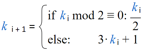
Pick a random integer > 1. It it is even, divide by 2. If it is odd, multiply by 3 and add 1. Do the same with the newly calculated value and so on. This is equivalent to the following series:

Collatz stated that whatever starting integer k0 > 1 you take, you will end up with calculating 1. Some curious people have tried this for all integers up to 1020 (at least) by using computers. So far, they haven’t found a single number that contradicted the conjecture.

But in math, this does not prove anything. It is still possible that some larger number exists, that will fail to comply. It may get trapped into an infinite cycle or simply diverge to infinity. So, it works like magic and no one in the world knows exactly why. A detailed explanation of the problem is provided in this YouTube video:

Actually, it is much easier to disprove the Collatz conjecture than proving it. It is enough to find just one number that contradicts the conjecture, and we are ready. No one managed to do that till now, but it doesn’t mean that we cannot try as well. It is quite unlikely to succeed because most probably the conjecture is true. But lets give it a try and hope to be lucky ;).

For that purpose, we will create a short program in Calcpad. Here is the code:

CollatzCheck(k; n) = $Repeat{k = switch(k ≡ 1; 1; k⦼2 ≡ 0; k/2; 3*k + 1) @ i = 1 : n}

That is all we need to do the job – one line of code. Here, k is the starting number and n is the maximum number of steps. According to the data from previous experiments, n is not expected to be larger than 10000. If we fail with this value we can try with a greater one. We can use the above function as follows:

CollatzCheck(100000000000001; 10000)

In return, we get 1 as expected. However, this function does not provide information about the number of steps required to finish (the stopping time). For that purpose, we will use a little hack and modify the function slightly. We will make it to divide by zero when we reach k = 1. This will force it to exit with error and report the value of i:

CollatzSteps(k; n) = $Repeat{k = switch(k ≡ 1; -1/0; k⦼2 ≡ 0; k/2; 3*k + 1) @ i = 1 : n}

After we call the new function:

CollatzSteps(100000000000001; 10000)

Error in “CollatzSteps(100000000000001; 10000)” on line [ ]: The function k = switch(k ≡ 1; -1/0; k⦼2 ≡ 0; k/2; 3*k + 1) is not defined for i = 252.

Now we know that it needed 252 steps to complete. However, this is not a nice way to return a result. But counting the number of steps and showing better output at the same time already require loops, as follows:

#def Collatz_Check$(k$; n$)
    #hide
    i = 0
    k_ = k$
    #repeat n$
        i = i + 1
        #if k_ ≡ 1
            #break
        #else if k_⦼2 ≡ 0
            k_ = k_/2
        #else 
            k_ = 3*k_ + 1
        #end if
    #loop
    #show
    #val
    #if k_ ≡ 1
        'Collatz check for <b>'k$'</b> <span class="ok">succeeded</span> after 'i' steps.
    #else
        'Collatz check for <b>'k$'</b> <span class="err">failed</span> after 'n$' steps.
    #end if
    #equ
#end def

This time we implemented a macro procedure to organize our code. We can use it for our purposes in the following way:

Collatz_Check$(100000000000001; 1000)

And here is the output:

Collatz check for 100000000000001 succeeded after 252 steps.

There is another improvement that we can apply. With a little modification, we can make the above procedure not only to count the steps, but also to plot them in the output:

#def Collatz_Plot$(k$; n$)
    #hide
    i = 0
    k_ = k$
    #show
    #val
    'Collatz check for <b>'k$'</b>:
    '<table>
    '<tr><td>Start -</td><td>&emsp;'k_'</td></tr>
    #repeat n$
        #hide
        i = i + 1
        #show
        #if k_ ≡ 1
            #break
        #else if k_⦼2 ≡ 0
            '<tr><td>/2 =</td><td>&emsp;'k_ = k_/2'</td></tr>
        #else 
            '<tr><td>*3 + 1 =</td><td>&emsp;'k_ = 3*k_ + 1'</td></tr>
        #end if
    #loop
    '</table>
    #if k_ ≡ 1
        'Check <span class="ok">succeeded</span> after 'i' steps.
    #else
        'Check <span class="err">failed</span> after 'n$' steps.
    #end if
    #equ
#end def

To make the output shorter and save some scrolling, we will use a smaller number to demonstrate this procedure:

Collatz_Plot$(11; 1000)

And this is what we obtain in return:

Collatz check for 11:

Start – 11
*3 + 1 = 34
/2 = 17
*3 + 1 = 52
/2 = 26
/2 = 13
*3 + 1 = 40
/2 = 20
/2 = 10
/2 = 5
*3 + 1 = 16
/2 = 8
/2 = 4
/2 = 2
/2 = 1

Check succeeded after 15 steps.

This is very useful to see how this sequence actually works. First, the expression 3*k + 1 transforms the odd number to even, that will be immediately halved (at least once). Second, if the latest is a multiple of 2n, we will have n consecutive downsteps, that may go much lower than the initial value. So, maybe we should ask the question: what is the distribution of n for all 2n multiples in a certain range and now often we will hit a multiple with larger n

However, if we want to check more numbers, it would be tedious to do it one by one. We should write another procedure that checks all integers in a given range:

#def Collatz_Check_Between$(k0$; kn$; n$)
    #hide
    k0 = max(k0$; 1)
    i = k0 - 1
    #repeat kn$ - k0 + 1
        i = i + 1
        k_ = CollatzCheck(i; n$)
        #if k_ ≠ 1
            #break
        #end if
    #loop
    #show
    #val
    #if k_ ≡ 1
        'Collatz check <span class="ok">succeeded</span> for all numbers between 'k0' and 'kn$'.
    #else
        'Collatz check <span class="err">failed</span> for <b>'i'</b> and 'n$' steps.
    #end if
    #equ
#end def

The above function can be used as given bellow:

Collatz_Check_Between$(2; 100000; 400)

After less than a second we get the result:

Collatz check succeeded for all numbers between 2 and 100000.

So, this is how we can use Calcpad to experiment with the Collatz conjecture. You can download the complete source code for the above examples from GitHub:

https://github.com/Proektsoftbg/Calcpad/blob/main/Examples/Mathematics/Collatz%20Check.cpd

If you still do not have Calcpad, you can download and install it for free from the following link:

https://calcpad.eu/download/calcpad-setup-en-x64.zip

Now you can use Calcpad to perform your own experiments. If you get lucky to disprove the Collatz conjecture, please share credits ;).

If you want to learn more about this spiky mathematical problem, there are various sources in the internet, you can start with:

https://en.wikipedia.org/wiki/Collatz_conjecture

https://mathworld.wolfram.com/CollatzProblem.html

How to calculate special functions with Calcpad

There are many special mathematical functions that are not defined by arithmetic expressions, but as a solution of some definite integral. Such are Gamma and related functions, Error function, Fresnel integrals, elliptic integrals, etc. Unlike some advanced mathematical packages as Octave, Maxima or Scilab, they are not implemented internally in Calcpad. However, for real numbers, you can easily define them in any worksheet by using the numerical integration procedures. Read this post further to learn how.

Gamma function

Gamma function is an extension of the factorial to the real and complex domains. For integer arguments it is defined by:

Γ(n) = (n – 1)!

For real and complex numbers it is usually defined by the Euler’s integral form:

However, this form is not convenient for calculations because of the infinite upper limit. Fortunately, the Gamma function can be also expressed as a definite integral with finite limits as follows:

It seems that this is what we need. For real z > 0, we can apply the embedded Tanh-Sinh adaptive integration to solve this by using the $Integral command. But if we try to do that, we will stumble upon another problem – the formula gets unstable for z < 1. We can solve this easily by using the identity for real z > 0:

Finally, we arrive at the following expression, that we can use for real positive values x:

It can be defined in Calcpad by the code bellow:

Γ(x) = $Integral{ln(1/t)^x @ t = 0 : 1}/x

If we plot it for x = 0.05 to 5, we will get the following graph:

To verify how it works, we tested the function for the calculation of several known values. The results are presented in the table below:

nxΓ(x) Expected Error
10.51.7724538509055162.50550506363359×10-16
21110
31.50.8862269254527581.25275253181679×10-16
42112.22044604925031×10-16
52.51.3293403881791388.3516835454453×10-16
632.00000000000000221.11022302462516×10-15
73.53.3233509704478461.069015493817×10-15
846.00000000000000661.03620815631681×10-15

The results are obtained for a target precision of 10-14, which is the default precision in Calcpad for numerical methods. The resulting relative error is equal to or less than 10-15.

Error function

Error function is defined by a definite integral of the Gaussian function as follows:

For real, positive values of z, we can use directly the above formula. It will not work for negative values in Calcpad because Calcpad cannot integrate backwards. In other terms, the upper bound of the integral should be greater than the lower bound.

However, we can use the identity: erf(-z) = –erf(z) to fix this, and it eventually leads to the following equation:

It can be defined in Calcpad by the code bellow:

erf(x) = 2*sign(x)/sqrt(π)*$Integral{e^-t^2 @ t = 0 : abs(x)}

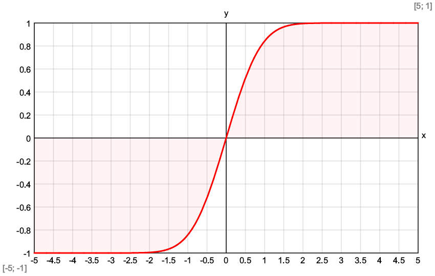
If we plot it for x = -5 to 5, we will get the following graph:

Again, we will check how it works by calculating the function for several points and estimating the relative error.

nxerf(x) Expected Error
10000
20.50.5204998778130470.5204998778130462.1329938237256×10-16
310.8427007929497150.8427007929497152.6349162927426×10-16
41.50.9661051464753110.9661051464753110
520.9953222650189540.9953222650189537.80808532624166×10-16
62.50.9995930479825560.9995930479825557.77472511244569×10-16
730.9999779095030020.9999779095030017.77173285381738×10-16

For the target precision of 10-14 the obtained relative error is close to the machine precision. Other functions like Fresnel integrals, Si, Ci, Shi, Chi, etc. can be defined in a similar way.

Html UI with Calcpad

Calcpad is a handy tool for writing engineering calculation notes. You can simply type your formulas and text (in quotes) on the left side and get your report calculated and formatted on the right. Then you can print it or send it to MS Word, Libre Office or a PDF file.

However, if you have a long and complicated problem or need to share it with other users, working directly with the source code is not the most practical way. First, there is a risk to damage the code by making inappropriate changes. Second, it may be difficult to identify what is input data and what is not, especially if you are not the author.

Basic input forms

That is why, Calcpad provides an option for easy creation of Html forms for data input. All you have to do is to put a question mark “?” wherever you need a value to be entered. After it, add the default value in curly brackets, as follows:

"Stress in Simply Supported Beam
'Length -'L = ? {5}m
'Cross section
b = ? {250}mm','h = ? {500}mm
'Loads -'q = ? {10}kN/m','N = ? {0}kN
...

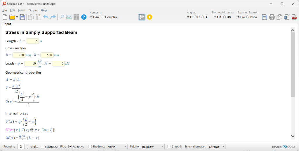
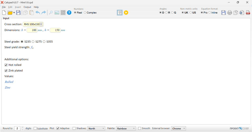
Then, press F4 or the “Compile to input form” button (on the left of the “Run” button) to generate the form. You will get the following result:

Calcpad will display the uncalculated Html output, where all question marks are replaced by input fields. The source code will be hidden and not accessible anymore. You will have to press again F4 or toggle the same button back to unlock it. Once in input mode, you can enter the input data safely and run the calculations by pressing F5.

Probably, you may not want to see all this uncalculated output during the input. For that purpose, Calcpad provides you with special switches to specify what to be visible on each stage:

#pre – the contents after the current line will be visible only in input phase;
#post – the contents will be visible only in results phase;
#hide – the contents will be hidden in both phases;
#show – the contents will be visible in both phases.

If you insert #post before “Geometrical properties”, you will hide the remaining contents during the input phase. Add some images, compile again, and you will get a nice and friendly input form, like the one bellow:

Advanced Html forms

Besides text input fields, Calcpad allows more advanced UI elements like selection lists, radio buttons and checkboxes. Unlike text fields, they are not generated automatically. You have to use Html to insert them. If you are not familiar with Html, you can use various online resources to learn the basics, like https://www.w3schools.com/html/

Unlike text fields, Calcpad does not support other UI elements natively. It can read values only from text fields. That is why, you should link all other elements to some “target” text fields. The latest will be used by Calcpad to fill the input data from the source UI elements, after the user makes some selection. This is performed automatically by predefined JavaScript code in the Calcpad Html template.

Although it looks a bit complicated, there is an easy way to start. Calcpad provides ready made code snippets in the Insert -> Html UI menu.

Then you can play with the generated code to see how it works and modify it according to your needs. We will use this approach to create a small example for selection of steel sections, material grade and fabrication method (cold formed or hot rolled) for the selected section.

Selection

Inserted code:

'Select an option: <select name="target1">
'<option value="11;12">x1; y1</option>
'<option value="21;22">x2; y2</option>
'<option value="31;32">x3; y3</option>
'</select>
'<p id="target1"> Values:'x = ? {21}','y = ? {22}'</p>

Modified code:

'Cross section: <select name="section">
'<option value="100;150">RHS 100x150</option>
'<option value="150;200">RHS 150x200</option>
'<option value="200;250">RHS 200x250</option>
'</select>
'<p id="section"> Dimensions:'b = ? {100}mm','h = ? {150}mm'</p>

Result:

Comments:

The select Html element must have an opening <select> and closing </select> tags. You can put inside as many options as you need. Each option also has opening and closing tags, which are <option> and </option>, respectively. Between them, you have to put the actual text that will appear in the list. The values should be specified inside the value="" attribute. You can have multiple values for each option. They must be numerical and separated by semicolons without spaces. Each option must include the same number of values as the number of the target input fields.

The target input fields must be enclosed with a paragraph Html element. It must have an id="" attribute that matches exactly the name="" attribute of the select element. You can make the default values for the input fields to be equal to the values of a certain option. Then, this option will be loaded by default at startup. If there is no matching option, the select element will be empty at startup.

Radio buttons

Inserted code:

'<p>Select: 
'<input name="target2" type="radio" id="opt1" value="1"/>
'<label for="opt1">option 1</label>
'<input name="target2" type="radio" id="opt2" value="2"/>
'<label for="opt2">option 2</label>
'...
'<p id="target2">Value -'opt = ? {2}'</p>

Modified code:

'<p>Steel grade:
'<input name="steel" type="radio" id="S235" value="235"/>
'<label for="S235">S235</label>
'<input name="steel" type="radio" id="S275" value="275"/> 
'<label for="S275">S275</label>
'<input name="steel" type="radio" id="S355" value="355"/> 
'<label for="S355">S355</label></p>
'<p id="steel" style="display:none;">'f_y = ? {235}MPa'</p>
'Steel yield strength:'f_y

Result:

Comments:

The basic principle is similar to the select element. All radio buttons must have a name that matches the id of the target paragraph. After a radio is clicked, the contents of its value="" attribute will be filled in the text input after “fy =“. The label next of each radio is specified by a respective “label” element. Its for="" attribute should correspond to the id of the radio. If you want to hide the text field from the form and leave only the radio buttons, you should add a style="display:none;" attribute to the target paragraph.

Checkbox

Inserted code:

'<p><input name="target3" type="checkbox" id="chk1" value="3"/>
'<label for="chk1">Checkbox 1</label></p>
'...
'<p id="target3">Value -'chk = ? {3}'</p>

Modified code:

'<p><input name="Rolled" type="checkbox" id="roll" value="1"/>
'<label for="roll">Hot rolled</label></p>
'<p id="Rolled" style="display:none;">'Rolled = ? {1}'</p>
Rolled

Result:

Comments:

Unlike radio buttons, each checkbox must have exactly one target paragraph with an input field inside. When the checkbox is checked, its value is filled in the target input field. If unchecked, the target input field is reset to zero “0“.

You can find the complete code of the above example in our GitHub repository:

https://github.com/Proektsoftbg/Calcpad/blob/main/Examples/Demos/Html%20UI.cpd

Comparison of three quadrature rules

Sometimes, in science and engineering, we need to calculate some definite integrals of the type:

It is equivalent to evaluating the area enclosed between the function graph and x-axis, within the interval [a, b]. There are some integrals (like elliptical, Fresnel, etc.) that cannot be expressed in analytical form. In such cases, we have to use numerical methods, also called quadrature rules. They approximate the integral by a finite sum like follows:

where xi are the abscissas of the nodes, where the function is calculated, and wi are the respective weights. Most quadrature rules use the same formula, but with different values for abscissas and weights.

Probably, most engineers are already familiar with Newton’s or Gauss formulas for numerical integration. However, there are other contemporary methods that can be more efficient for this purpose.

In this post, we will compare three quadrature rules for numerical integration. They will be applied to the same function, and with the same number of nodes. The calculations will be performed with Calcpad, as follows:

Test function (half-circle):

Theoretical value of the integral:

Number of nodes: n = 5

Boole’s rule

This is one of the Newton-Cotes‘ family of quadrature formulas, with order of n = 4. Nodes are located at equal spacing h, and weights are calculated by approximating the function with Lagrange polynomials.

Spacing – h = 0.5

AbscissasOrdinates
x1 = -1y1 = f(-1) = 0
x2 = -0.5y2 = f(-0.5) = 0.86603
x3 = 0y3 = f(0) = 1
x4 = –x2 = 0.5y4 = f(0.5) = 0.86603
x5 = –x1 = 1y5 = f(1) = 0

Integral:

Error:

Scheme:

Gauss-Legendre’s formula

This is the most simple Gaussian quadrature formula. The function is approximated by Legendre polynomials in the interval of [-1; 1]. Abscissas are determined as the roots of the respective polynomials, so the nodes are not equally spaced.

AbscissasOrdinatesWeights
x1 = -0.90618y1 = f(-0.90618) = 0.42289w1 = 0.23693
x2 = -0.53847y2 = f(-0.53847) = 0.84265w2 = 0.47863
x3 = 0y3 = f(0) = 1w3 = 0.56889
x4 = –x2 = 0.53847y4 = f(0.53847) = 0.84265w4 = w2 = 0.47863
x5 = –x1 = 0.90618y5 = f(0.90618) = 0.42289w5 = w1 = 0.23693

Abscissas and weights are calculated by the following equations:

Integral:

IG = 2·w1·y1 + 2·w2·y2 + w3·y3 = 2·0.23693·0.42289 + 2·0.47863·0.84265 + 0.56889·1
IG = 1.5759

Error:

Scheme:

Tanh-Sinh quadrature

This is one of the double exponential integration formulas, proposed by Takahasi and Mori (1974).

Boundary of the interval – ta = 1

Step:

Parameter – tk = –ta + (k – 1) ·h

Formula for calculation of abscissas:

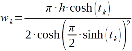
Formula for calculation of weights:

AbscissasOrdinatesWeights
x1 = x(1) = -0.95137y1 = f(-0.95137) = 0.30806w1 = 0.11501
x2 = x(2) = -0.67427y2 = f(-0.67427) = 0.73848w2 = 0.48299
x3 = x(3) = 0y3 = f(0) = 1w3 = 0.7854
x4 = –x2 = 0.67427y4 = f(0.67427) = 0.73848w4 = w2 = 0.48299
x5 = –x1 = 0.95137y5 = f(0.95137) = 0.30806w5 = w1 = 0.11501

Integral:

Value:

IDE = 2·w1·y1 + 2·w2·y2 + w3·y3 = 2·0.11501·0.30806 + 2·0.48299·0.73848 + 0.7854·1
IDE = 1.5696

Error:

Scheme:

Summary of the results

The relative errors, from the above three quadrature rules are presented in the following chart:

We can see that the Gaussian quadrature rule is much more precise than the Newton-Cotes’ one of the same order, which is expected. However, Tanh-Sinh quadrature shows the best results from all three. And this is not by chance. According to Wikipedia, this is probably the most efficient numerical integration rule ever known.

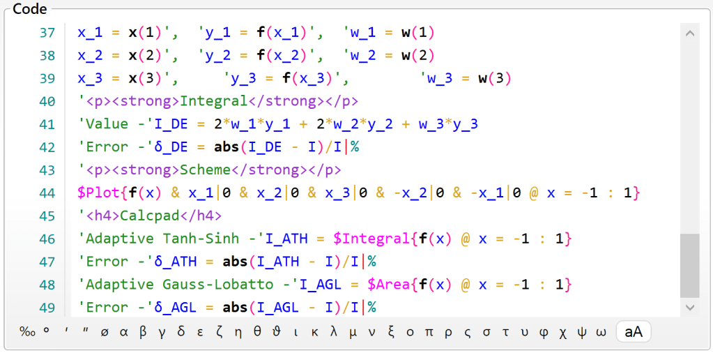
That is why, it’s adaptive version is implemented in Calcpad as the main numerical integration method ($Integral command). Alternatively, you can use the adaptive Gauss-Lobatto quadrature ($Area command). It is much slower, but unlike the Tanh-Sinh one, it works for functions that are not smooth and continuous.

For the above example, both of them provides extremely high accuracy, that is comparable to the floating point precision of the double (float64) data type:

You can download the Calcpad source file from GitHub:

https://github.com/Proektsoftbg/Calcpad/blob/main/Examples/Mathematics/Numerical%20Integration.cpd

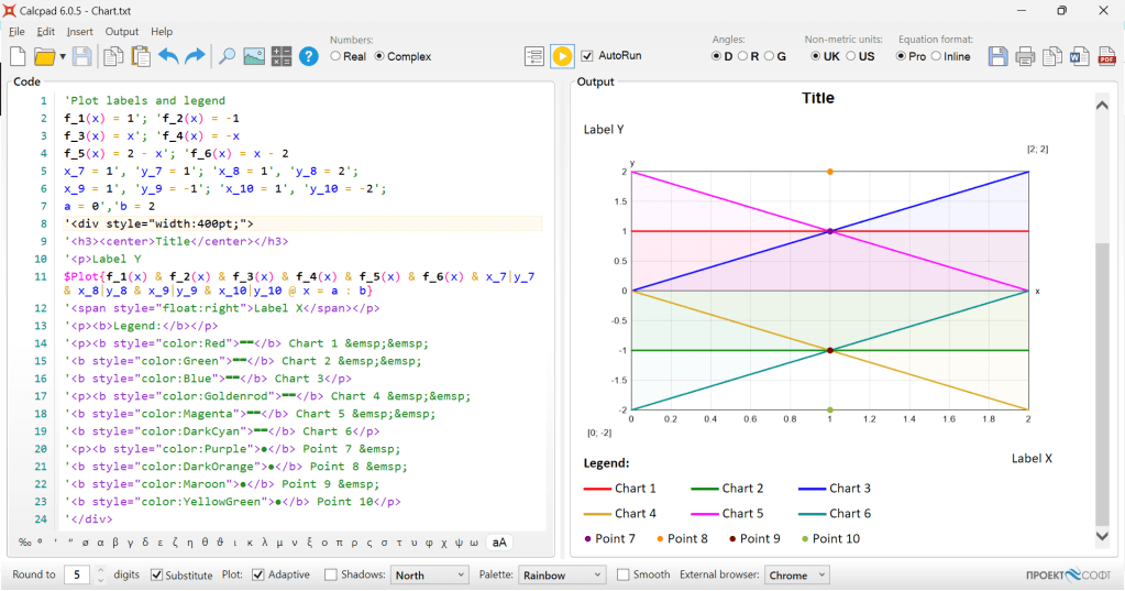
How to add title, labels and legend to a Calcpad plot?

Calcpad does not provide options to add titles, axis labels and legends to function plots like in Excel. However, you can decorate your plots with these attributes by your own, by using a little Html.

Bellow, you can find a sample code that you can use as a boilerplate. Since chart colors are predefined, they will be the same for all your future plots:

'<div style="width:400pt;">
'<h3><center>Title</center></h3>
'Label Y
$Plot{f_1(x) & f_2(x) & f_3(x) & f_4(x) & f_5(x) & f_6(x) & x_7|y_7 & x_8|y_8 & x_9|y_9 & x_10|y_10 @ x = a : b}
'<p style="float:right">Label X</p>
'<p><b>Legend:</b></p>
'<p><b style="color:Red">▬▬</b> Chart 1 &emsp;&emsp; 
'<b style="color:Green">▬▬</b> Chart 2 &emsp;&emsp; 
'<b style="color:Blue">▬▬</b> Chart 3</p>
'<p><b style="color:Goldenrod">▬▬</b> Chart 4 &emsp;&emsp; 
'<b style="color:Magenta">▬▬</b> Chart 5 &emsp;&emsp; 
'<b style="color:DarkCyan">▬▬</b> Chart 6</p>
'<p><b style="color:Purple">●</b> Point 7 &emsp; 
'<b style="color:DarkOrange">●</b> Point 8 &emsp; 
'<b style="color:Maroon">●</b> Point 9 &emsp; 
'<b style="color:YellowGreen">●</b> Point 10</p>
'</div>

And here is how it looks inside Calcpad:

If you have less charts, you can delete the extra lines. Also, there is an option for points, if both x and y are fixed. If you have any questions, please do not hesitate to ask them right away.

Units in empirical formulas

There are many formulas in structural design codes, that are empirical and if you enter them in Calcpad “as are”, you will not obtain the results in the expected units. Moreover, there are even formulas, that are not dimensionally correct and won’t calculate. Lets take for example the shear resistance without reinforcement, according to Eurocode 2. It is calculated by the following formula:

  VRd,c = (CRd,c k (100 ρl   fck)1/3 + k1σcp) bwd (6.2a)

Here, fck and σcp are in MPa, so, we will end up with MPa1/3 + MPa, which does not have physical meaning and cannot be calculated. The k factor is equal to:

  k = 1 + sqrt(200/d) ≤ 2.0

If d is in mm, we will get: 1 + mm-0.5, which also does not make any sense.

On the other hand, the minimum resistance is:

  VRd,c = (vmin + k1σcp) bwd (6.2b), where

    vmin = 0.035k3/2 fck1/2

How can we solve this problem?

Obviously, we have no choice, except to manually compensate for the missing dimensions. For example the value of “200” in the formula for k is actually in mm. So, we will have k = 1 + sqrt(200mm/d) and get a dimensionless result as expected.

If we apply the same approach for the other formulas, we will obtain the following little program for calculation of shear resistance without reinforcement to Eurocode 2:

'Section width -'b_w = 250mm
'Effective height -'d = 450mm
'Main reinforcement ratio -'ρ_l = 0.02
'Characteristic concrete strength -'f_ck = 25MPa
'Partial safety factor for concrete -'γ_c = 1.5
'Design concrete strength -'f_cd = f_ck/γ_c
'Normal stress -'σ_cp = 0MPa
'Factors:'k_1 = 0.15', 'C_Rd,c = 0.18/γ_c
k = min(1 + sqr(200mm/d); 2)
v_min = 0.035*k^(3/2)*sqr(f_ck)*MPa^0.5|MPa
'Shear resistance
'<p class="ref">(6.2a)</p>
V_Rd,c = (C_Rd,c*k*(100*ρ_l*f_ck)^(1/3)*MPa^(2/3) + k_1*σ_cp)*b_w*d
'Minimum shear resistance 
'<p class="ref">(6.2b)</p>
V_Rd,c = (v_min + k_1*σ_cp)*b_w*d

When you run the above program in Calcpad, the results will look as follows:

You should not worry about that formulas do not look exactly as in the design codes. It is far more important to give the correct results as it can be easily verified.

What’s new in Calcpad 5.8 and later?

In the last several months, Calcpad was subjected to continuous improvement, driven by the efforts of its developers and the help of the community. In this post, we will make a short review of the most important changes.

1. Modules

If you have a simple and short worksheet, it is definitely easier to keep it all in a single file. But imagine that you have to build an entire library for design of timber structures. And each worksheet should start with identical content for selection of materials and cross sections. Then, it would be better to put this part in a separate module and reference it from all other worksheets. Now, you can do this in Calcpad, using the following code:

#include filename.cpd

If the file is in the same folder, you can enter only the filename, otherwise you must specify the full path. This is better than copying one and the same text in all worksheets. You can also select which part of the module is local and global by inserting the respective keywords: “#local“, “#global“. Local parts will not be included into the external module.

2. String variables and macros

This is a good way to further organize your code and avoid repetitions at a module level. You can assign a piece of code to a string variable. Then, you can insert it wherever you like, by simply writing the name instead of the whole text.

The difference between variables and macros is that macros have parameters, and variables don’t. On the other hand, both can be inline of multiline. All names must and with the “$” symbol and can include letters, numbers and underscore “_”. You can use the following syntax:

Inline string variable:

#def variable_name$ = content

Multiline string variable:

#def variable_name$
'content line 1
'content line 2
'...
#end def

Inline macro:

#def macro_name$(param1$; param2$; ...) = content

Multiline macro:

#def macro_name$(param1$; param2$; ...)
'content line 1
'content line 2
'...
#end def

This is a really powerful feature that can save a lot of work. It allows you to expand the Calcpad functionality with features that never existed before. For example, you can create Html “shortcodes” for faster and better formatting:

#def b$(x$) = <strong>x$</strong>
#def i$(x$) = <em>x$</em>
#def sup$(x$) = <sup>x$</sup>
#def sub$(x$) = <sub>x$</sub>
#def err$(x$) = <span class="err">x$</span>
'Usage:
'<p>b$(Check): i$(f)sub$(yk) = err$(2) kN/cmsup$(2)</p>

Result:
Check: fyk = 2 kN/cm2

Another interesting example is the following general design check routine:

#def check$(x$; x_max$)
    #if x$ ≤ x_max$
        'The check is satisfied:'x$'≤'x_max$'✓
    #else
        '<p class="err">The check is not satisfied:'x$'&gt;'x_max$'✖</span></p>
    #end if
#end def

Usage:

σ = 280MPa','σ_lim = 250MPa
check$(σ; σ_lim)
τ = 120MPa','τ_lim = 0.58*σ_lim
check$(τ; τ_lim)

Result:
σ = 280 MPa , σ lim = 250 MPa
The check is not satisfied: σ = 280 MPa > σlim = 250 MPa
τ = 120 MPa , τ  lim = 0.58·σ lim = 0.58·250 MPa = 145 MPa
The check is satisfied: τ = 120 MPaτ lim = 145 MPa

Modules, string variables and macros are parsed at preprocessor stage. Calcpad scans the code and rewrites the names with the actual contents. As a result, it generates “unwrapped” source code. If you check the respective checkbox you will see it in the output window, instead of the calculation results. It will also show automatically if any error occurs in preprocessing.

3. Angle units

In the latest versions, native angle units are available for use:
°, deg – degrees;
– minutes = degrees/60; 
– seconds = minutes/60;
rad  – radians = π / 180 degrees;
grad  – grades = 10 / 9 degrees;
rev – revolutions = 360 degrees.

You can convert between angle units and combine them with others to create composite ones like “rad/s” and “rev/min“. Angle units are accepted by all trigonometric functions. They override all other settings, made in the Calpad UI or by using “#deg“, “#rad” and “#grad” keywords in the code. Inverse trigonometric functions can optionally return the results with units, if you define the variable: “ReturnAngleUnits = 1“.

4. C/C++ style operators

Some relational operators in Calcpad use mathematical notation symbols like , , , , which are not available on computer keyboards. Although Calcpad provides buttons for insertion, this is still slower than typing. That is why, we introduced an alternative C/C++ like syntax that uses only keyboard symbols as follows:

OperatorSymbolAlt syntax
equal==
unequal!=
less or equal<=
greater or equal>=

The alternative symbols are replaced with the original ones while typing.

5. Calcs suppression with #noc

Previously, there were only two visibility control keywords regarding equations:
#equ – displays the equation and the result;
#val – displays only the final result without the equation.

Recently, we added one more option:
#noc – displays only the equation, without the result;

It not only hides the results, but also suppresses the calculations. This allows you to use Calcpad as a simple equation editor for faster typing of formulas. Unlike MathML and LaTeX, which use special syntax, Calcpad formats raw, simple text equations. At the end, you can export the entire content to MS Word or Libre Office with MathType/Math formatted equations.
6. Integration with Tanh-Sinh quadrature

Double exponential quadrature (Takahasi & Mori, 1974) is one of the most efficient numerical integration algorithms. In our tests, it demonstrated outstanding performance, compared to other popular methods: Integration-test-results.pdf. It is also adaptive and very accurate. The only problem is that the function must be continuous and smooth. However, due to its efficiency, we decided to include it as a second method, using the “$Integrate” command.

The original algorithm has been improved further by Michashki & Mosig (2016) and Van Engelen (2022). In Calcpad, we made additional enhancements by precomputing and caching the abscissas and weights.

In all cases, you can continue using the old “$Area” command, which is more general purpose. It is powered by the famous adaptive Gauss-Lobatto-Kronrod quadrature by Gander & Gautschi (2000).

7. Improved formatting

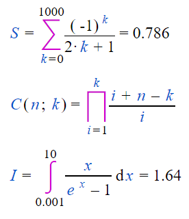
Sums, products and integrals are now formatted with the respective large symbol and limits on bottom and top. That gives the reports more professional feel and look. For example:

S = $Sum{(-1)^k/(2*k + 1) @ k = 0 : 1000}
C(n; k) = $Product{(i + n - k)/i @ i = 1 : k}
I = $Integral{x/(e^x - 1) @ x = 0.001 : 10}

are formatted as follows:

8. Input fields defaults

In the previous versions, default values for input fields were specified by clicking the respective question marks in the code. When you saved the file, they were appended consequently at the end. This made uncomfortable using external editors like Notepad++ for writing Calcpad code. After introducing modules and macros, it was almost impossible to match the values with the corresponding input fields.

That is why, we changed the approach and made the default values to be added immediately after the question marks. You must enclose them with curly brackets, like: “a = ? {2}“. You can also override the values inside modules and macros by specifying the values as in the following example:

#include abc.cpd #{4; 5; 6}
d = a + b + c

If abc.cpd has the following contents:

a = ? {1}
b = ? {2}
c = ? {3}

The result will be:
a = 4
b = 5
c = 6
d = a + b + c = 4 + 5 + 6 = 15

9. Custom rounding

You can also override the global rounding settings for certain parts of your code, by using the “#round n” keyword. Replace n with the number of digits after the decimal point (from 0 to 15).

10. Pausing and step by step execution

If you have long calculations, you can pause the solution by pressing the “Pause/Break” key or “Ctrl + Alt + P” from the keyboard. Then, you can resume it with “F5“. Also, you can define breakpoints in your code by using the “#pause” and “#input” keywords. They correspond to two types of breakpoints:
#pause – stops the solution at the current line and displays the avalable results;
#input – stops at themcurrent line and renders an input form.

On the next #input, it will calculate and show the results before the current one and render the next input form. Sometimes, engineers need to see some intermediate results before entering more data. For example, when you design a RC beam, you calculate the required main reinforcement from bending ULS. After that, you select some actual reinforcement and use it further for SLS checks like deflections, crack widths, etc.

11. Performance and optimization

In the last few versions, we made important optimizations to improve Calcpad performance, as follows:

  • UI responsiveness – it is not lagging anymore on large files;
  • text processing and parsing – string splitting is replaced by the more effective memory spans wherever possible;
  • function caching – now it works faster, but consumes much less memory;
  • compiling – “constant folding” was introduced for faster execution;
  • units – units arithmetic performance was enhanced by 20% – 30%.

You can learn more about the new features from the Calcpad documentation:

calcpad-readme.pdf

5 reasons to choose math worksheets over Excel spreadsheets for structural calculations

Although there are plenty of software nowadays, engineers still have to develop custom calculations to solve specific problems. Some may still make them “by hand”, but most engineers use some kind of software for that.

The problem is that in most cases, we have to document our calculations and collect them in design reports or calculation notes. And it would be also very good, if we could give them professional look and feel. The other issue is to make the calculations reusable, in case we have similar projects in future.

Apparently, a peace of paper and pencil would not do the job anymore. Even a simple hand calculator (except for quick estimates). What we need is a suitable software for that purpose, but what?

To my experience, the most widely used solution for custom engineering calculations is Excel. At the same time, it is probably the most inappropriate for the job. But it is not actually an Excel fault. In general, it is a great software, very mature and high quality, but for tabular data. I myself usе it quite a lot for bills of materials and construction cost calculations. Spreadsheets are the best for simple formulas that have to be repeated on multiple rows/columns.

However, structural design algorithms are tree-like in nature, not tabular. Even if a tree data structure can fit in a table, this is not the optimal solution. It has some issues that cannot be neglected. During the years, I had to write a lot of structural design spreadsheets on Excel, as well as math worksheets on software like MathCAD or Calcpad. Over time, I found some important reasons to prefer the math approach over Excel spreadsheets:

1. Formulas are built by referencing cells.

It is slow to write and difficult to check and follow, especially for the longer ones. “M = FL + qL^2/2″ is much easier to type and more readable than “= D2A3 + C1A3^2/2″. It is like obfuscation of the actual formula. For longer calculations, it gets even harder. Imagine that you have 1000 lines (rows) of calculations and your formula uses some cells at row 1, 500, 200, 700, 900, etc. You will have to scroll up and down multiple times to find the required cells to be referenced. Of course, you can use named cells, to improve readability, but it requires additional work.

2. Formulas are hidden inside the cells.

That makes the printed report a real black box for the checking engineer. There is an option to make them visible, but without formatting they are difficult to read. The best option is to write them once again with MathType. Besides it is a double work, you can mistype something and there is no guarantee that the formulas you see, are the same inside the cells. Also, variable substitution in formulas is not available in this case. So, Excel spreadsheets are prone to errors.

3. You cannot apply units of measurement to values and use them in formulas.

You can write units of measurement in the next cell, but you cannot attach them to values and they will not take part in your calculations as it happens in math software. So, you must include the proper conversion factors manually in all of your formulas. Otherwise, you will simply get incorrect results.

4. It is difficult to define your own custom functions.

You must use VBA programming, which is not an option for a newbie. In math software, this is a piece of cake. You can simply type f(x) = 2*x^3 – … Also, it is very easy to plot a function graph directly from its equation. In Excel, you must calculate it in multiple cells and then, plot the respective range. If you have discontinuities or infinities and if you are not quite familiar with the function properties in advance, you can easily miss them and end up with incorrect graph.

5. It is almost impossible to branch the solution path and the report contents.

There are a lot of cases in structural design when the solution continues in completely different ways, depending on some intermediate checks. In systems like Calcpad, you can just add if-else if-else-end if condition blocks and put different formulas, text, and images in each one. In Excel, you can achieve limited results with intensive use of VBA.

So, even if you are an experienced spreadsheet developer and user, it is worth to give the math approach a try. Calcpad is perfect for this purpose, because it is lightweight, fast, easy to learn and free.

How to calculate square/cubic root by hand?

Today, technologies make everything easy and fast. And sometimes, when we see the ancient marvels of engineering, we wonder: “How they designed this without computers”? And the answer is: “with knowledge, inspiration and hard work”.

However, being almost irreplaceable, computers makes us more and more adjective. Our brains become lazy and we are losing some knowledge and skills. Such is the manual calculation of root. It is so easy and elegant, so I will share it here for the sake of the good old math science.

Square root

Let’s calculate x = √a first. By squaring both sides and moving a to the left side, we obtain the following equation:

x2a = 0

This is an equation of type f(x) = 0 and we can solve it numerically, using the Newton’s method, as follows:

  1. Start with initial guess: x0. It is good to be close to the solution, so you can use the nearest exact root.
  2. Calculate the next approximation of the root by the equation: x1 = x0f(x0)/f′(x0)
  3. Continue the iterations by using the previous result to estimate a new one:
    xn+1 = xnf(xn)/f′(xn).
  4. Stop when you reach the desired precision.

In the above formulas, f(x) is the function and f′(x) is the first derivative. In our case:
f(x) = x2a
f′(x) = 2x

If we substitute the above equations into the Newton’s iterative formula, we get:
xn+1 = xn − (xn2a)/2xn
xn+1 = (xn + a/xn)/2

Now, lets use it to calculate √a = ?, for a = 5. We will start with an initial guess of x0 =√4 = 2.

1st iteration: x1 = (x0 + a/x0)/2 = (2 + 5/2)/2 = 2.25
2nd iteration: x2 = (x1 + a/x1)/2 = (2.25 + 5/2.25)/2 = 2.2361
3rd iteration: x3 = (x2 + a/x2)/2= (2.2361 + 5/2.2361)/2 = 2.2361

After the second iteration, we have 5 correct significant digits, which is quite sufficient for most cases.

Cubic root

We will use the same approach, as follows:
f(x) = x3a
f′(x) = 3x2
xn+1 = xn − (xn3a)/3xn2
xn+1 = (2xn + a/xn2)/3

Let’s see how it works for 3√7. Our initial guess is: x0 = 3√8 = 2.

1st iteration: x1 = (2x0 + a/x02)/3 = (2·2 + 7/22)/3 = 1.9167
2nd iteration: x2 = (2x1 + a/x12)/3 = (2·1.9167 + 7/1.91672)/3 = 1.9129
3rd iteration: x3 = (2x2 + a/x22)/3 = (2·1.9129 + 7/1.91292)/3 = 1.9129

Again, we managed to find it after two iterations. We can also use Calcpad to create a tiny program for that:

It is interesting that after just 4 iterations, the Newton’s method finds 16 correct significant digits, which is the limit precision for most computers. We also calculated the root by three different methods which gived the same result.