
There are many special mathematical functions that are not defined by arithmetic expressions, but as a solution of some definite integral. Such are Gamma and related functions, Error function, Fresnel integrals, elliptic integrals, etc. Unlike some advanced mathematical packages as Octave, Maxima or Scilab, they are not implemented internally in Calcpad. However, for real numbers, you can easily define them in any worksheet by using the numerical integration procedures. Read this post further to learn how.
Gamma function
Gamma function is an extension of the factorial to the real and complex domains. For integer arguments it is defined by:
Γ(n) = (n – 1)!
For real and complex numbers it is usually defined by the Euler’s integral form:

However, this form is not convenient for calculations because of the infinite upper limit. Fortunately, the Gamma function can be also expressed as a definite integral with finite limits as follows:

It seems that this is what we need. For real z > 0, we can apply the embedded Tanh-Sinh adaptive integration to solve this by using the $Integral command. But if we try to do that, we will stumble upon another problem – the formula gets unstable for z < 1. We can solve this easily by using the identity for real z > 0:

Finally, we arrive at the following expression, that we can use for real positive values x:

It can be defined in Calcpad by the code bellow:
Γ(x) = $Integral{ln(1/t)^x @ t = 0 : 1}/xIf we plot it for x = 0.05 to 5, we will get the following graph:

To verify how it works, we tested the function for the calculation of several known values. The results are presented in the table below:
| n | x | Γ(x) | Expected | Error |
| 1 | 0.5 | 1.772453850905516 | 2.50550506363359×10⁻¹⁶ | |
| 2 | 1 | 1 | 1 | 0 |
| 3 | 1.5 | 0.886226925452758 | 1.25275253181679×10⁻¹⁶ | |
| 4 | 2 | 1 | 1 | 2.22044604925031×10⁻¹⁶ |
| 5 | 2.5 | 1.329340388179138 |  | 8.3516835454453×10⁻¹⁶ |
| 6 | 3 | 2.000000000000002 | 2 | 1.11022302462516×10⁻¹⁵ |
| 7 | 3.5 | 3.323350970447846 |  | 1.069015493817×10⁻¹⁵ |
| 8 | 4 | 6.000000000000006 | 6 | 1.03620815631681×10⁻¹⁵ |
The results are obtained for a target precision of 10-14, which is the default precision in Calcpad for numerical methods. The resulting relative error is equal to or less than 10-15.
Error function
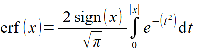
Error function is defined by a definite integral of the Gaussian function as follows:

For real, positive values of z, we can use directly the above formula. It will not work for negative values in Calcpad because Calcpad cannot integrate backwards. In other terms, the upper bound of the integral should be greater than the lower bound.
However, we can use the identity: erf(-z) = –erf(z) to fix this, and it eventually leads to the following equation:
It can be defined in Calcpad by the code bellow:
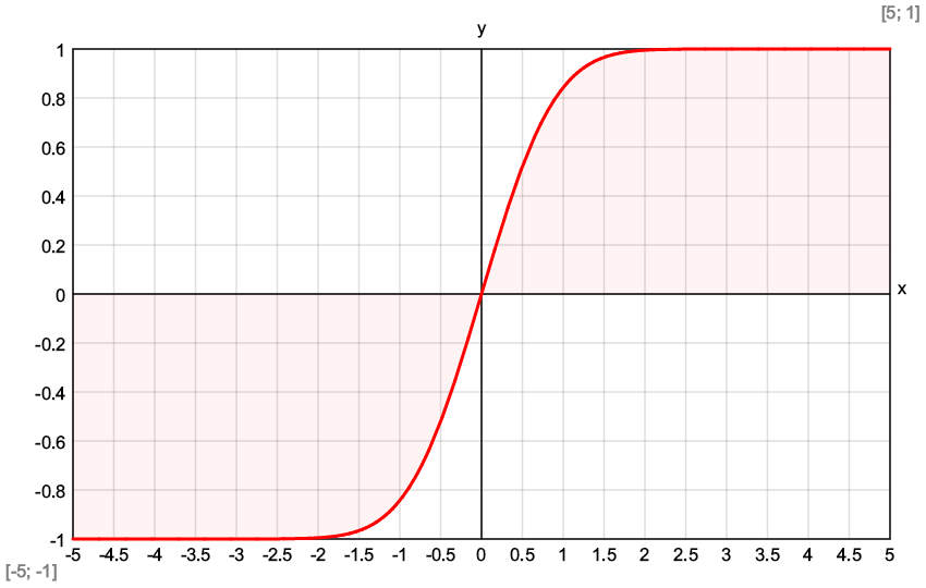
erf(x) = 2*sign(x)/sqrt(π)*$Integral{e^-t^2 @ t = 0 : abs(x)}If we plot it for x = -5 to 5, we will get the following graph:
Again, we will check how it works by calculating the function for several points and estimating the relative error.
| n | x | erf(x) | Expected | Error |
| 1 | 0 | 0 | 0 | 0 |
| 2 | 0.5 | 0.520499877813047 | 0.520499877813046 | 2.1329938237256×10⁻¹⁶ |
| 3 | 1 | 0.842700792949715 | 0.842700792949715 | 2.6349162927426×10⁻¹⁶ |
| 4 | 1.5 | 0.966105146475311 | 0.966105146475311 | 0 |
| 5 | 2 | 0.995322265018954 | 0.995322265018953 | 7.80808532624166×10⁻¹⁶ |
| 6 | 2.5 | 0.999593047982556 | 0.999593047982555 | 7.77472511244569×10⁻¹⁶ |
| 7 | 3 | 0.999977909503002 | 0.999977909503001 | 7.77173285381738×10⁻¹⁶ |
For the target precision of 10-14 the obtained relative error is close to the machine precision. Other functions like Fresnel integrals, Si, Ci, Shi, Chi, etc. can be defined in a similar way.
